How Regularizers Fix Dumb Solutions

A dumb solution

To get home from São Carlos to Araxá, I pass through Ribeirão Preto. It’s the shortest and most convenient route. Going through Brasília, Brazilian capital, is a bad idea - I’d still get home, but I’d walk many kilometers more.

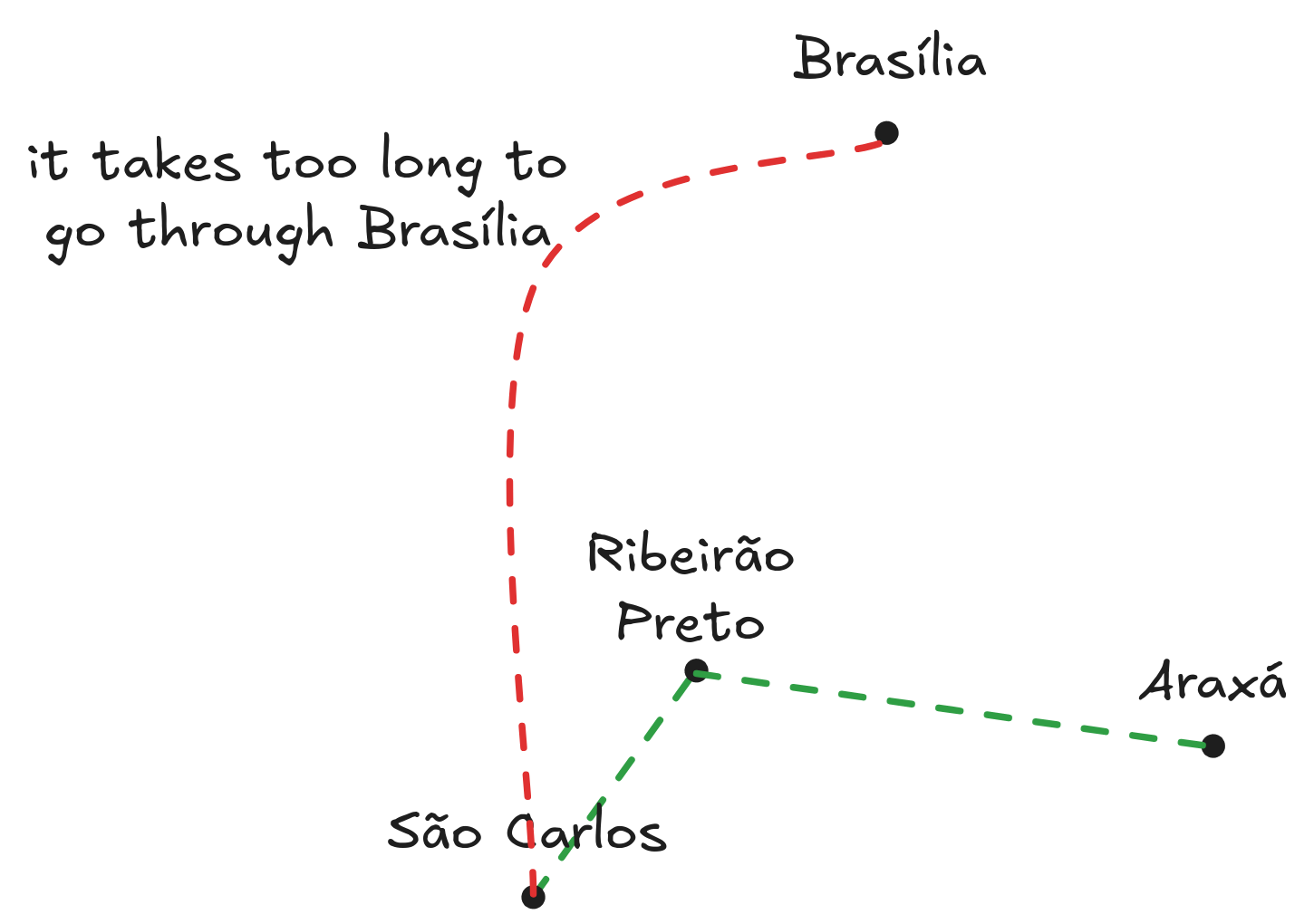
Not only those two paths exist, but many more. Similarly, there exists many functions that passes through all points in a graph.

But some are inefficient, just like going through Brasília. Regularizers help us find simpler solutions.

Take polynomial functions, for example. Their empirical risk is the sum of squared errors - the distances between predicted values and actual ones. Essentially, the empirical risk measures how good the curve fits the data. In the plot below, both models have similar empirical risk. Which one should we choose?

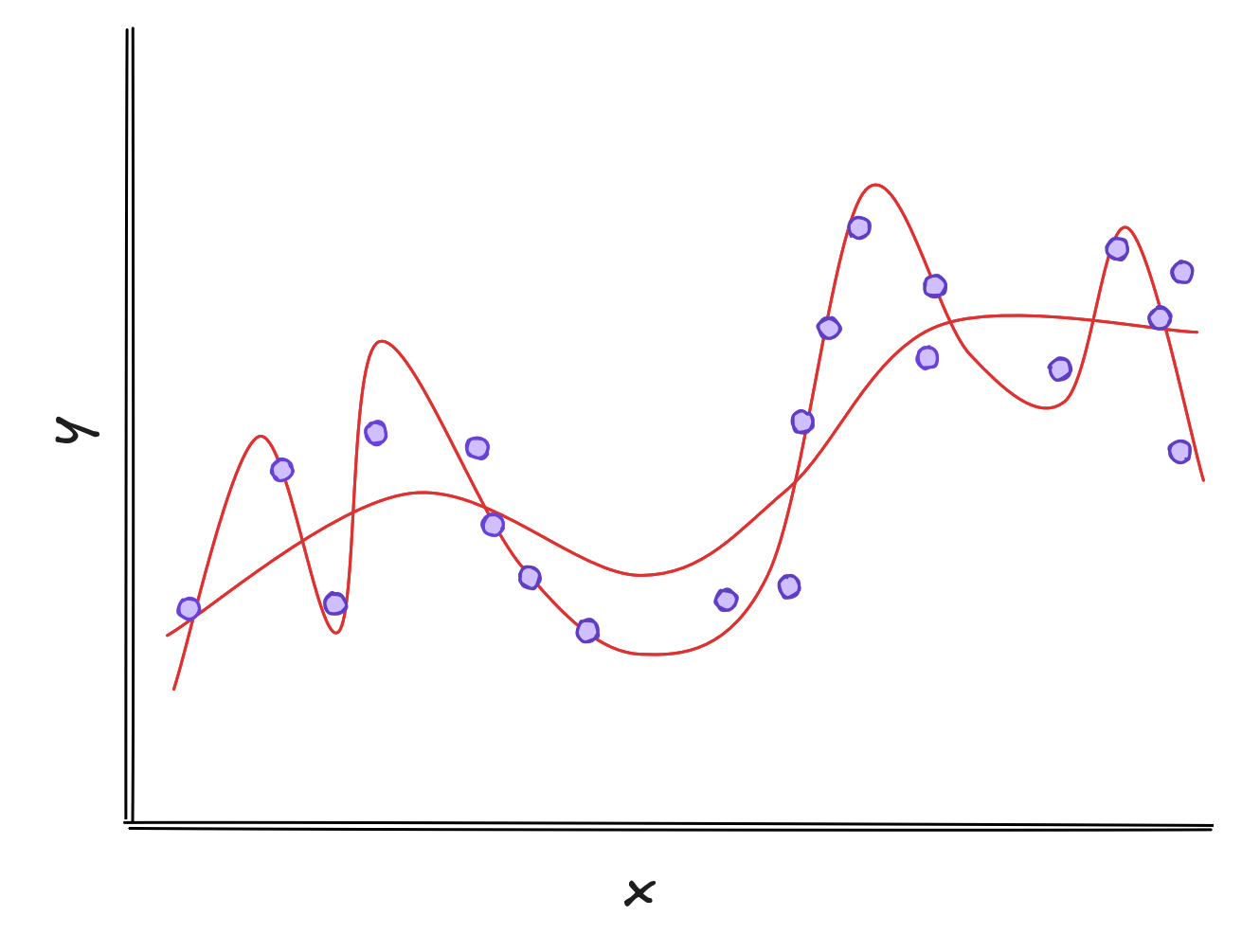
The squiggly line might perform well on the training dataset, but it is just like a student that memorizes homework questions instead of learning how to solve each one. When taking the test, the student is shocked to learn that not a single question is identical to the homework.

Likewise, the wiggly curve fails on new examples. The smoother one, however, generalizes better and handles unseen data more reliably.

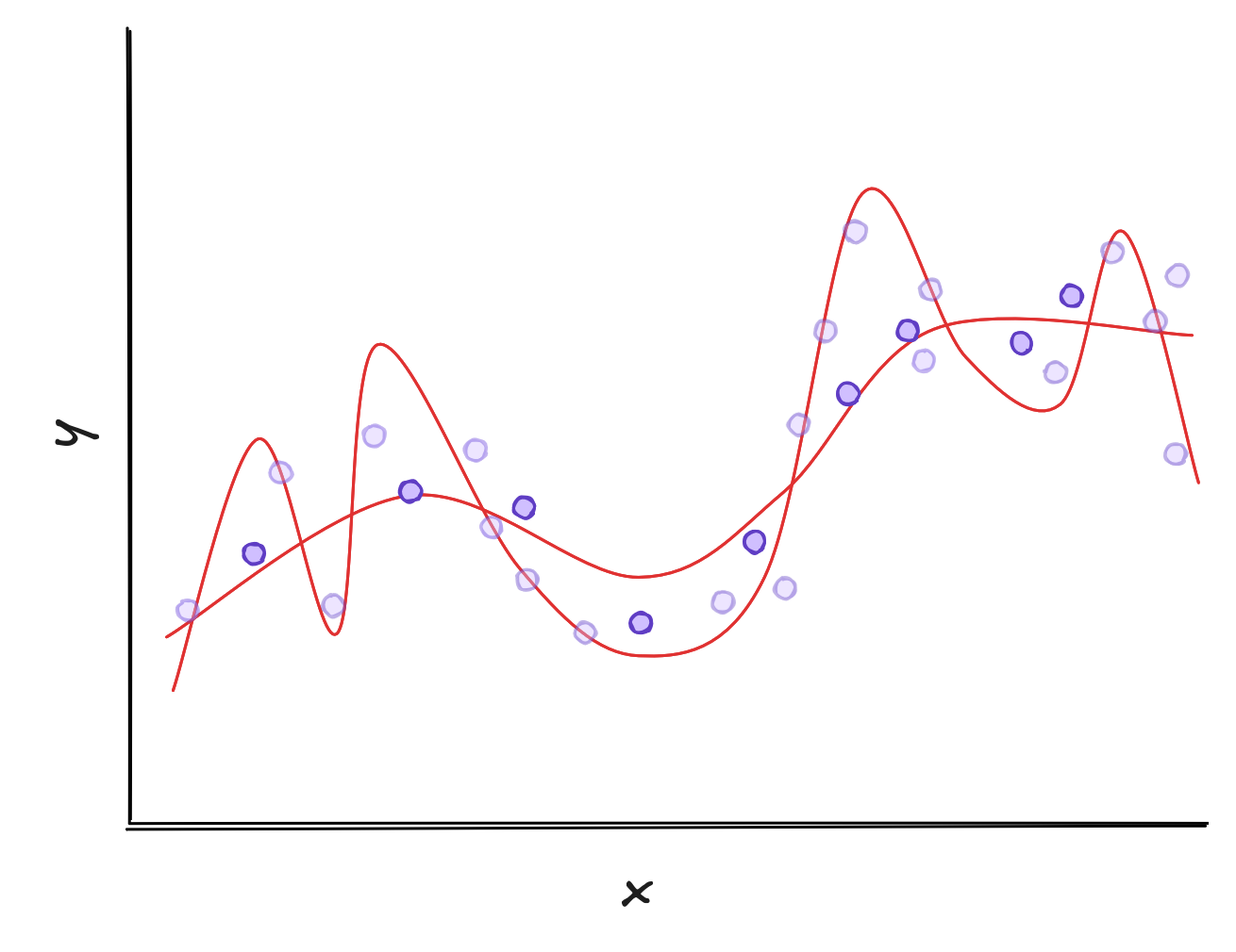
In Machine Learning, we say the wiggly curve overfitted Overfitting happens when there are too many possibilities to choose a model from.

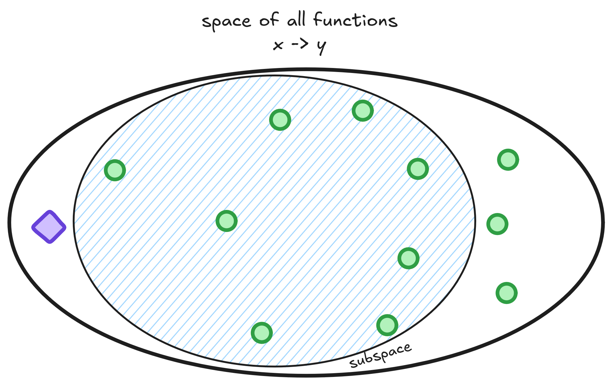
There are better ways of visualizing overfitting than thinking about squiggly lines. Think of the space of functions - all possible mappings from $x$ to $y$. We should pick linear functions, polynomials, or neural networks to train our model - a smaller subspace within the space of all functions.

During training, we search for functions inside this subspace - shown as green points - that are closest to the Oracle, marked in purple. The Oracle is a hypothetical function that perfectly captures the true relationship between $x$ and $y$. We then pick the function with the lowest empirical risk.

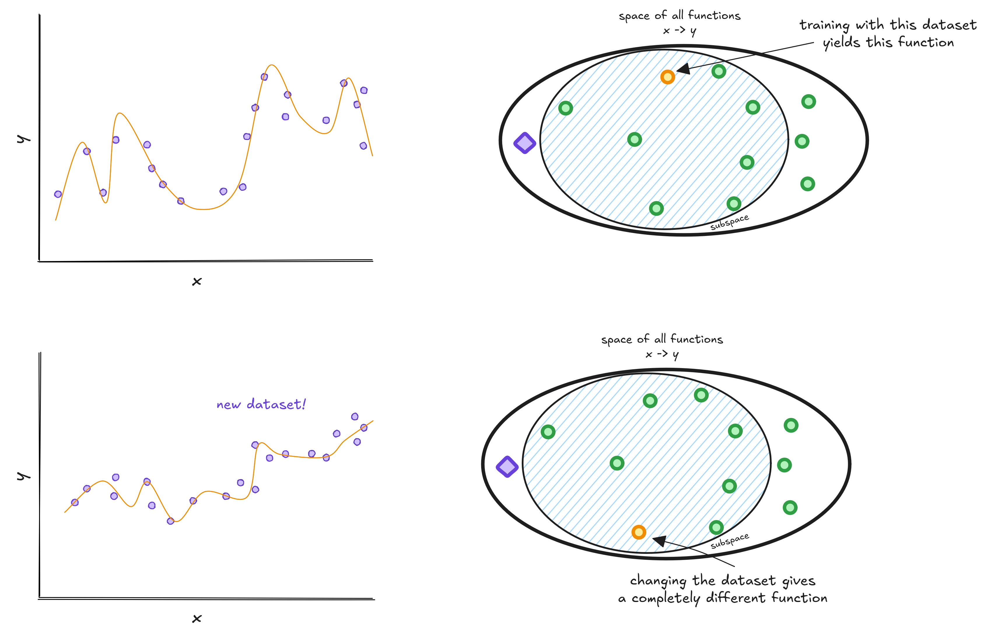
When we choose a complex model, like a neural network or a high-order polynomial, the subspace becomes too large - and finding the best model is like finding a needle in a haystack.

The final model depends heavily on the training data - it can end up with low, medium, or high true risk depending on the dataset. In other words, it has high variance.

Choosing a simpler model is not always an options, since they can be too simple.

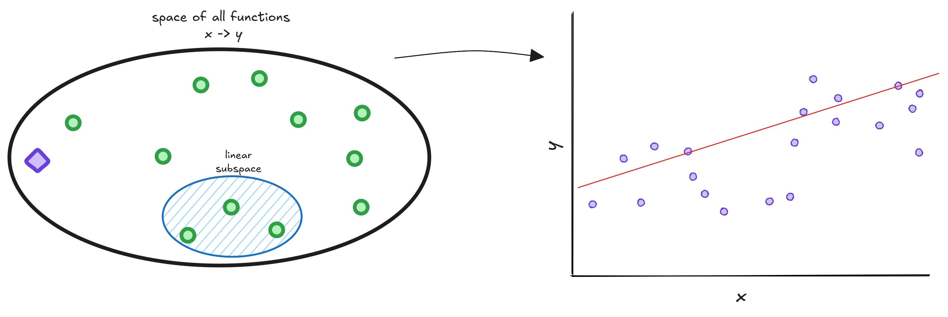
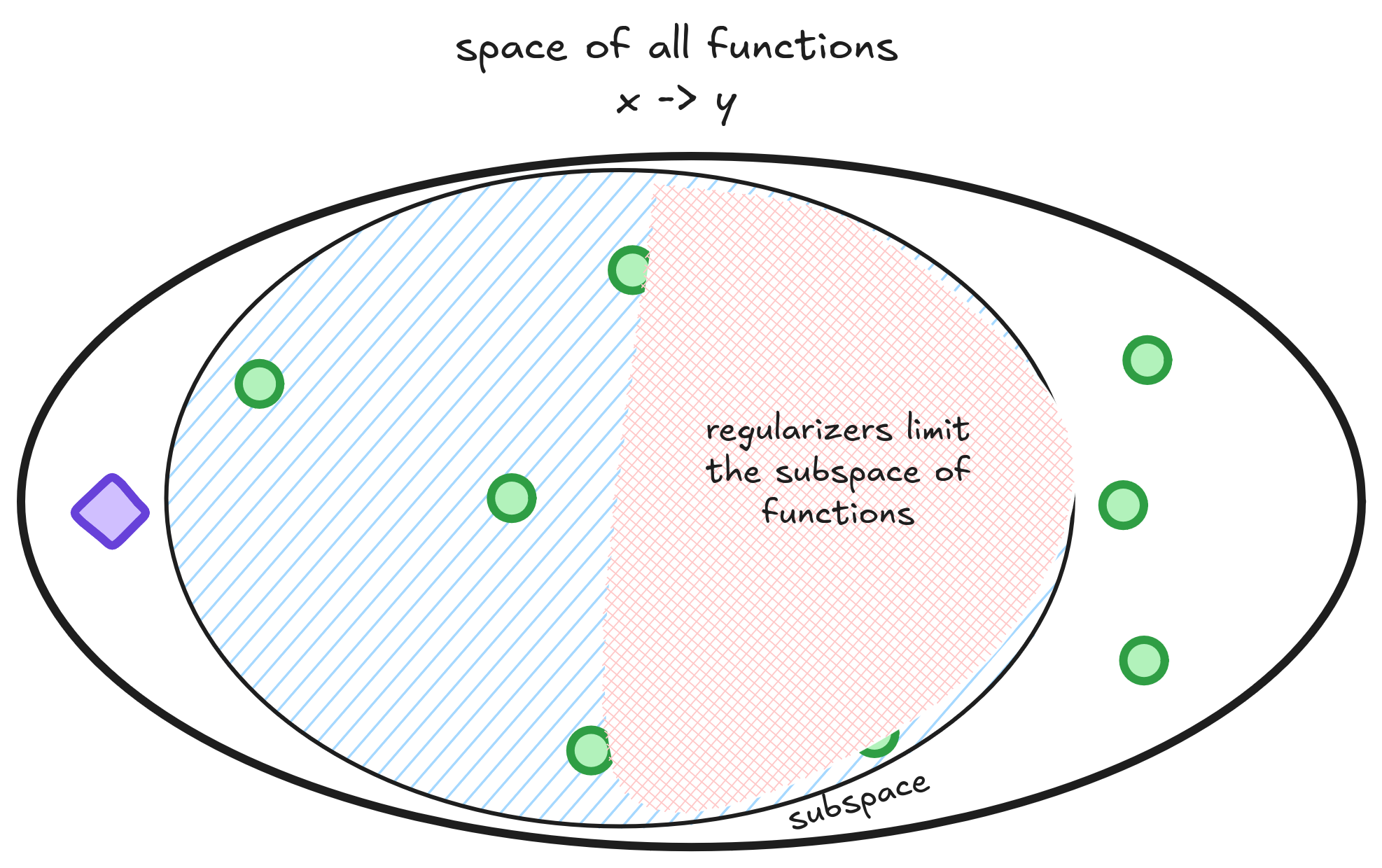
The idea behind regularizers is to restrict this big subspace in such way that dumb solutions like passing through Brasília are no longer an option.

Creating a regularizer

We didn’t like the wiggly functions because they overfit. A good regularizer should penalize the parts of those functions that lead to overfitting.

A first-order polynomial predicts values using a line: $y = f(x) = ax + b$, where $a$ and $b$ are the coefficients. A second-order polynomial adds a quadratic term: $y = ax^2 + bx + c$. Adding more terms creates higher-order polynomials. Our squiggly curve is one of these high-order polynomials with coefficients $a, b, c, d...$. We can use the whole alphabet if needed.

The problem with high-order polynomials is their large coefficients. When coefficients get extreme, the function can vary wildly and fit every point perfectly.

• High Coefficients Values: $f(x) = 30x^3-23x^2-16x+10$
• Low Coefficients Values: $f(x) = 0.4x^3-1x^2-0.8x+10$

We’ve seen that curvy lines and big coefficients cause overfitting. Intuitively, smaller coefficients - which create smoother curves - work better.

This intuition is called prior knowledge. For example, it’s why we avoid routes with many cities when traveling-the more cities, the longer the trip.

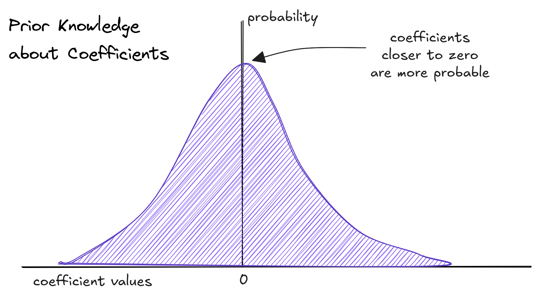
Here, the prior is: "most coefficients should be close to zero." We express this using a bell-curve (Normal) probability distribution, which favors coefficients near zero.

To restrict the large function space and reduce variance, we add prior knowledge to the usual regression optimization.

Now, we minimize

The penalty term is the standard norm of the coefficients $||\text{coefficients}||^2$ which increases as the coefficients get larger. A norm is just a function that take a vector outputs a number. Here, the standard norm is the square root of the sums of the coefficients squared.

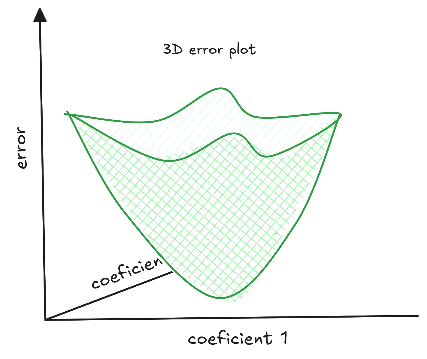
In traditional regression, we find coefficients that minimize empirical risk. The plot shows how the error changes with different coefficients - the minimal risk is at the lowest point.

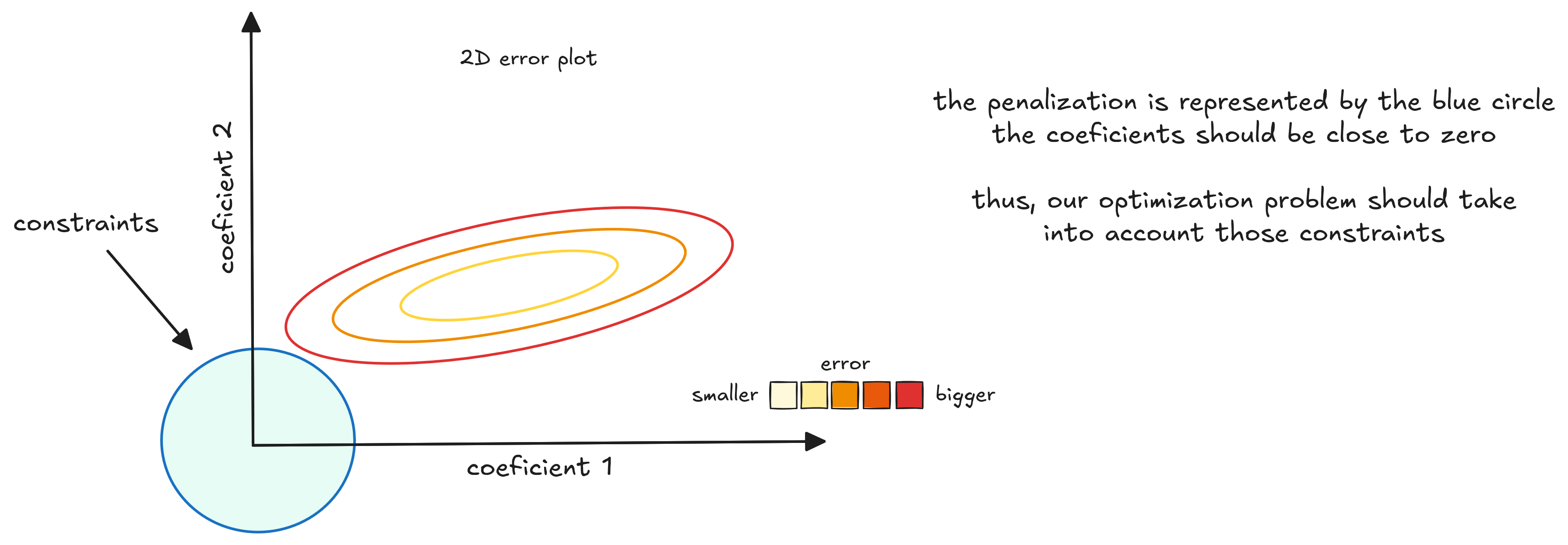
Now, we search coefficients that minimize our risk and are close to zero. With this constraint, visualizing in two dimensions makes it easier to understand.

The 3D plot is represented by ellipses, which are contours showing different error levels. Greener ellipses mean smaller errors. The circle at the origin represents the regularizer. We want to find coefficients that minimize the error and stay inside this circle.

We can solve this optimization using Gradient Descent. This algorithm moves downhill, following the steepest descent until it reaches a minimum. Here, that minimum is where the error curve meets the regularizer’s circle.

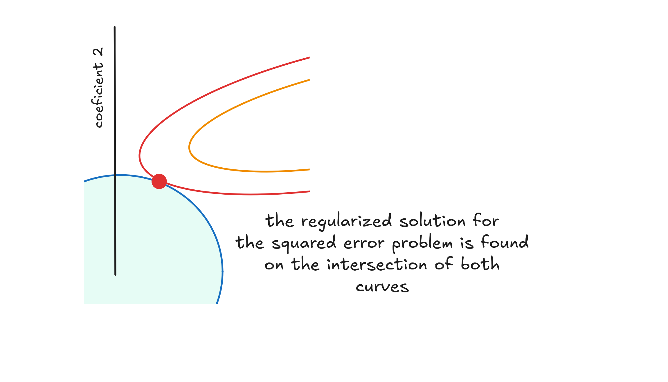
This minimum gives us coefficients that minimize squared error while staying close to zero.

Thus, the Normal Prior over the coefficients of the model gives this regularizer. Can we ajust the regularizer for different problems?

Tweaking the Regularizer

I ommited an important factor all along - one of the most important ones.

If the function space is very large or complex, we might want stronger regularization. Otherwise, a smaller penalty usually works fine.

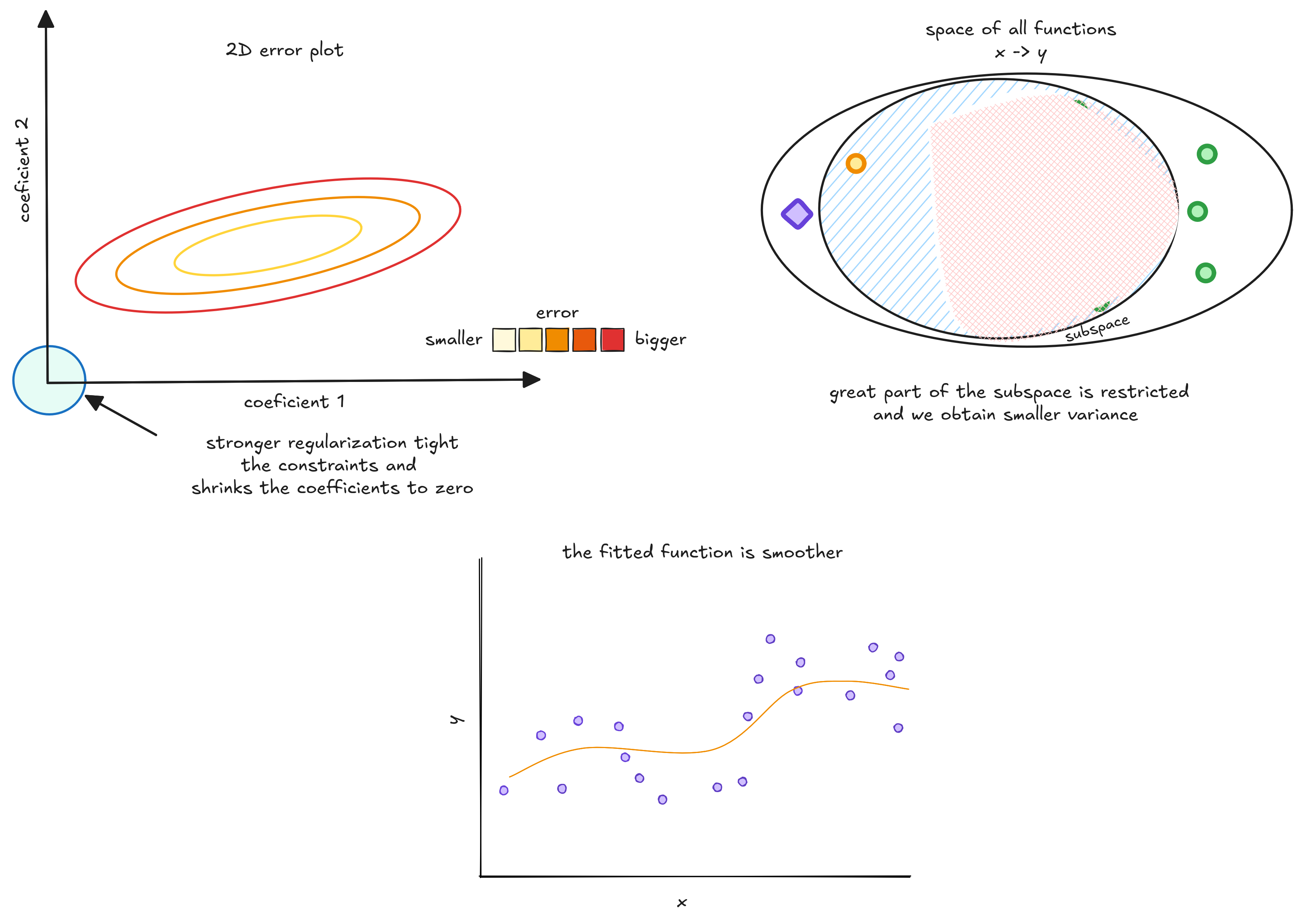
This is controlled by a term called lambda ($\lambda$), which sets the regularization strength. When lambda is close to zero, regularization is weak.

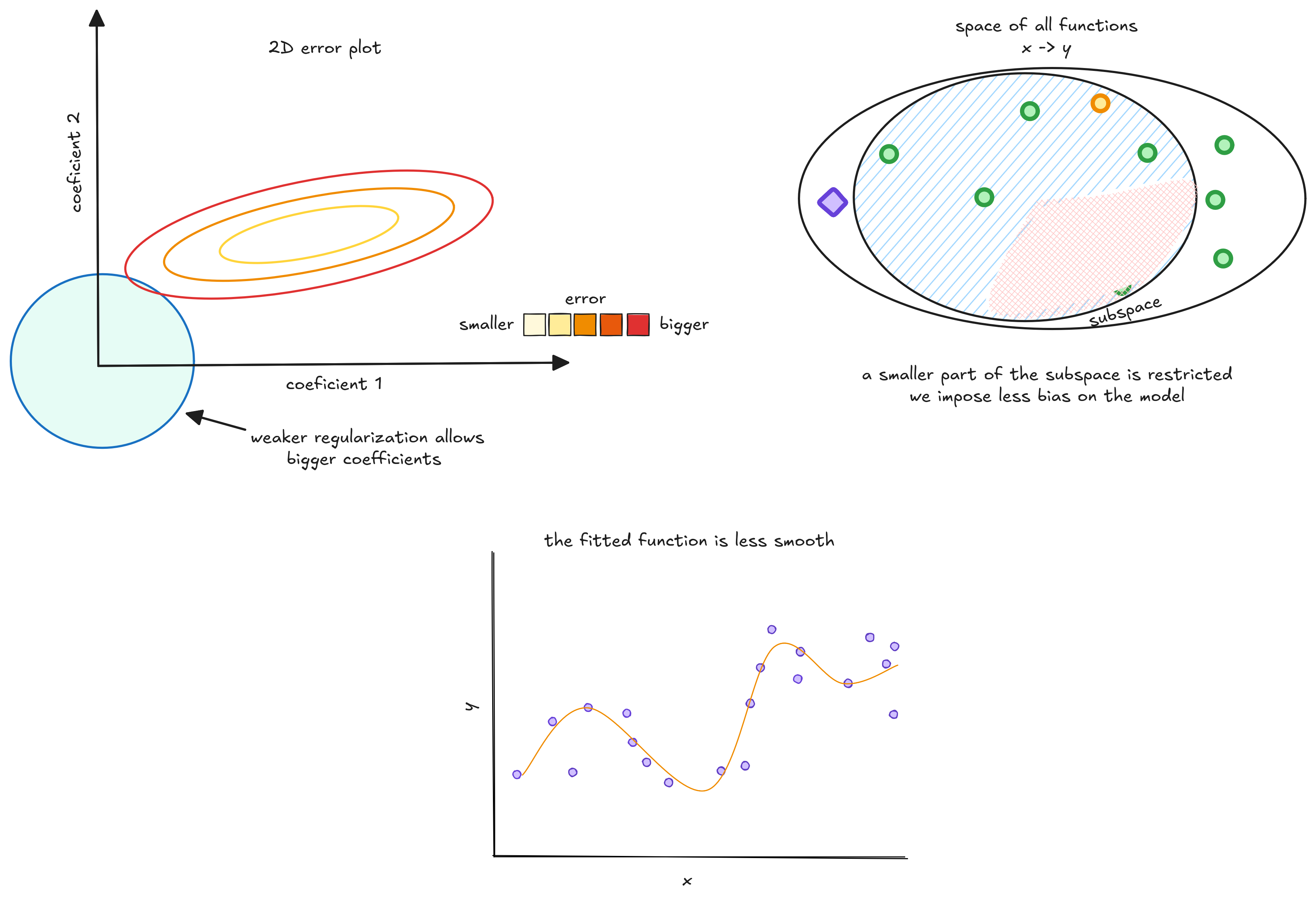
As lambda increases, regularization gets stronger, pushing weights closer to zero.

This lambda is commonly called an hyperparameter of the model. A hyperparameter is one parameter of the model engineers and scientists should set to make sure training goes right. And there are many techniques for it.

This is only one way of regularizing machine learnig models. At least we are not going through Brasília now.